library(ggplot2)
library(foreign)
library(car)
library(dplyr)
library(rpart)
library(fpc)
library(ggplot2)
library(Rmisc)
library(extrafont)
library(extrafontdb)

Are evangelicals are a monolith?

A lot of outsiders have begun to wonder if evangelicals are truly a monolithic bloc or are there some cracks beginning to form in what we believe an evangelical to be. I wanted to take a look at that by using a technique that is helps to sort a group into similar cases, also known as a cluster. These clusters are created using an algorithm and will help to divide evangelicals up into camps.

Data Cleaning

gss <- read.dta("D:/reltrad.dta", convert.factors = FALSE)
gss <- subset(gss, year >= 2010)
evan <-subset(gss, evangelical == 1)

The first thing I have done is used the RELTRAD coding scheme employed by Steensland et al (2000) to create a unified measure of evangelicalism. Here is a link to my github with that syntax for both Stata and R:. In addition I am just using data from the General Social Survey from 2010 to 2014. That is the three most recent waves of the GSS. The subgroup of evangelicals is sufficiently large (about 1500). I am going to do a bunch of cleaning behind the scenes now to get the data in a usable format. To see the full coding and cleaning syntax I have posted it here.

I’m going to create a dataframe to just do the clustering, called test. Here’s the variables that are included.

test <- select(evan, age, literal, attnd, male, tolerance, abortion, gaymarriage, gaysex, repubid, welfare, military, environment, drugs, educ)

I can’t have any missing data for the clustering to work properly. I have a handful of cases where age is missing, as well as education. I am going to use some prediction modeling to make a guess at both the age and education for the missing values.

age_fit <- rpart(age ~ educ + attnd + male + tolerance + abortion + gaymarriage + gaysex + repubid + welfare + military + environment + drugs, data = test[!is.na(test$age), ],
method = 'anova')
test$age[is.na(test$age)] <- predict(age_fit, test[is.na(test$age), ])

educ_fit <- rpart(educ ~ age + attnd + male + tolerance + abortion + gaymarriage + gaysex + repubid + welfare + military + environment + drugs, data = test[!is.na(test$age), ],
method = 'anova')
test$educ[is.na(test$educ)] <- predict(educ_fit, test[is.na(test$educ), ])

Clustering

Now, it’s time to run the clustering. But how many clusters should I use?

set.seed(555)
wss <- (nrow(test)-1)*sum(apply(test,2,var))
for (i in 2:15) wss[i] <- sum(kmeans(test,
                                     centers=i,iter.max=1000,algorithm="MacQueen")$withinss)

plot(1:15, wss, type="b", xlab="Number of Clusters",
     ylab="Within groups sum of squares")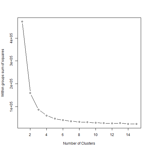

Using the graph it becomes apparent that the jump from 2 to 3 clusters still gives us a good deal of utility, but that moving to four clusters gives us a lot less. Let’s stick to three.

k<-kmeans(test, centers=3,iter.max=1000,algorithm="MacQueen")
k$size

## [1] 597 557 418

k$centers

##        age   literal     attnd      male tolerance  abortion gaymarriage
## 1 51.70015 0.5979899 0.6155779 0.4237856 0.4108319 0.1825796  0.06365159
## 2 31.68223 0.5385996 0.6429533 0.3788151 0.4240575 0.1579892  0.09694794
## 3 71.72727 0.6028708 0.6420455 0.4043062 0.3360447 0.1315789  0.03588517
##       gaysex  repubid   welfare  military environment     drugs     educ
## 1 0.11055276 4.216080 0.4003350 0.2881072   0.3763261 0.4103853 13.10720
## 2 0.15978456 4.168761 0.3776182 0.2998205   0.3997606 0.4111311 13.39677
## 3 0.07655502 4.270335 0.3915470 0.2838915   0.3197767 0.3979266 12.47060

So, we have three decently sized centers. That’s one of the advantages of MacQueen clustering. And we can see that the clusters have broken down really nicely into three age brackets with one cluster having the average age of 32, another having the average age of 53, and the third cluster is 73.

Before I go on, I have to note something. I know that in a typical clustering scenario you would want to standardize all your variables into a singular range, typically 0-1. However, this exercise was really meant to assess three generations of evangelicals and note the changes between those generations. Because of that the clustering is basically being swamped by the age variable.

Let’s visualize those three age clusters.

dp = discrproj(test, k$cluster)
test$clustname<-k$cluster
test$clustname<-factor(test$clustname)
ggplot(test, aes(dp$proj[,1], dp$proj[,2], color=factor(test$clustname)))+geom_point(pch=19,size=2)+ggtitle("Cluster Visualization")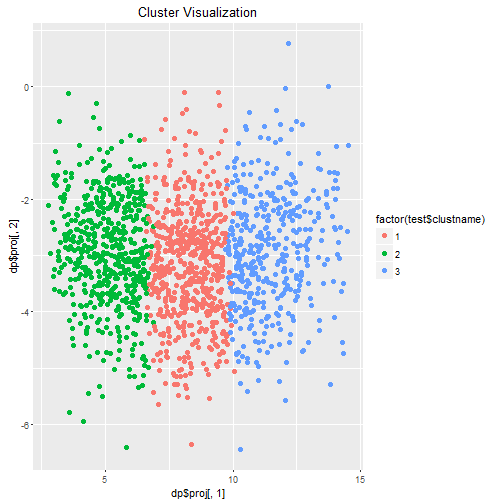

ggplot(test, aes(dp$proj[,1], dp$proj[,2], color=factor(test$literal)))+geom_point(pch=19,size=2)+facet_grid(clustname~.)+ggtitle("How Is Literalism Dispersed Through the Clusters")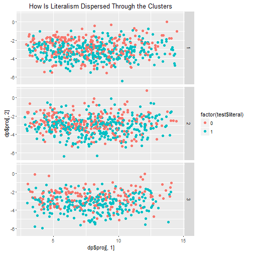

These visuals do look really nice, but because I am clustering on so many factors a two dimensional plot doesn’t really convey how the clusters actually look. We can tell that they are logically distributed across the x axis, however.

Results

Let’s start visualizing our results. I want to be able to tell two things.

1. Are evangelicals alike? Do each of the three clusters have the same opinions on government? Church attendance? The Bible?
2. How different are evangelicals than the general population?

Here’s how to read the charts. A dot represents the mean for each group. The lines extending out each side of the dot are the 84%* confidence intervals. If the lines for a cluster overlap the lines for another cluster then we cannot say that they have statistically different opinions on the subject.

*The 84% confidence interval for comparing means has become the standard measure for this application. While in other instances we rely on 95% CIs, recent writing in statistical theory have concluded that the 95% threshold is much too conservative. To read more click here.

The vertical dashed line you will see in the following graphs represents the mean of the entire GSS sample, not just evangelicals.

Religious Behavior

Let’s take a look at two religious behaviors. Believing in a literal Bible and church attendance.

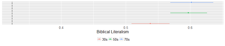
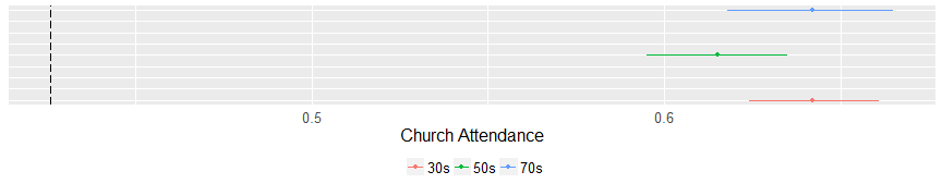
There are no surprises here. Evangelicals are much more likely to believe in a literal Bible and the youngest cluster in the analysis is less likely to believe that the Bible is literally true. The same is true of church attendance. No matter the age, evangelicals attend church at basically the same rate. Which is much more frequently than the general populace.

Tolerance

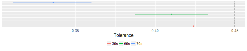
Now this is an intersting finding. The three clusters are distinct in the area of political tolerance. The older cluster is statistically less tolerant than the other two. Even more interesting is that the youngest cluster of evangelicals is not statistically more or less tolerant than the overall sample in the GSS. Maybe there are some differences forming here.

Social Issues

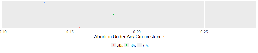
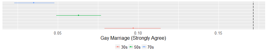
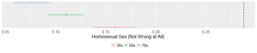
On the issue of abortion, evangelicals are united and distinct from the average American. The mean of no cluster is higher than 18% in favor of abortion under any circumstance. On the issue of gay marriage a similar pattern emerges. Evangeilcals are opposed to gay marriage and are far away from the average American. However, there is a small (but important) distinction on the issue of homosexual sex. The youngest cluster is more likely to say that homosexual is “not wrong at all” and this is statistically distinct from both other clusters.

Party Affiliation

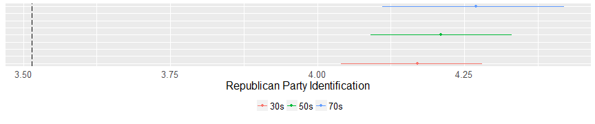According to these findings, evangelicals are pretty cohesive on their party affiliation. None of the clusters are ideologically distinct. However, they is a great distance between evangelical’s ideology and everyone else’s. According to these findings an evangelical is 10% more Republican than the average American.

Spending Issues

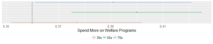
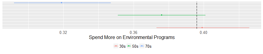
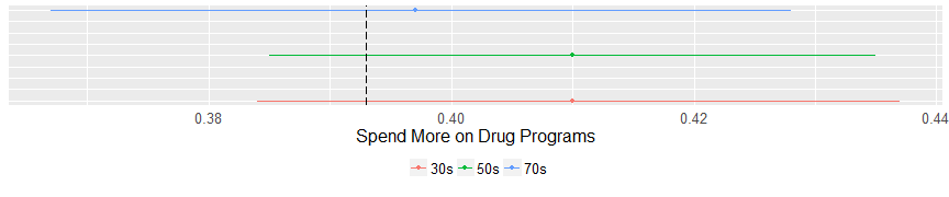
A few interesting things here. On the issue of welfare spending the middle cluster (those in their 50s) are more likely to favor spending on welfare programs than both the other two clusters and the general population. That’s an unusual finding. In regard to the environment, the older cluster (those in their 70’s) are less likely to support spending federal money but the other two clusters have an opinion on environment funding that is not different than the general population. On drug programs evangelicals all look alike and are no different than the general population.

Concluding Thoughts

So, are evangelicals a monolith? On matters of religiosity the answer is clearly yes. They attend church frequently and they have a very high view of the bible, which makes them distinct from the general population. Younger evangelicals are as tolerant as the average American while middle aged and older evangelicals are not. On social issues the younger set is showing signs of moving toward the center on issues of homosexuality but on abortion, evangelicals are in lock step. Which is also true in regard to political party affiliation. on taxing and spending older evangelicals oppose spending to the greatest degree but there are more moderate views among the other two groups on spending on the environment.

In fact, evangelicals are distinct and different than the general population but have achieved a remarkable amount of internal coherence.

I had to supress a lot of syntax to make this more readable. For full coding syntax visit my Github page