
library(ggplot2)
library(foreign)
library(gridExtra)
library(RColorBrewer)
library(choroplethr)
library(choroplethrMaps)
library(viridis)
library(DT)
library(knitr)
library(dplyr)
I got the county level voting datafile from here
I got the 2010 religious census data from here
vote <- read.csv("D:/2016_election/pres16results.csv", stringsAsFactors = FALSE)
vote$fips <- gsub("(?<![0-9])0+", "", vote$fips, perl = TRUE)
census <- read.dta("D:/2016_election/relcensus.dta", convert.factors = FALSE)
merge <- merge(census, vote, by=c("fips"))
suburbs <- read.csv("D:/2016_election/suburb.csv")
merge <- merge(merge, suburbs, by=c("fips"))
pres <- filter(merge, cand_name == "Donald Trump" | cand_name == "Hillary Clinton")
trump <- filter(merge, cand_name == "Donald Trump")
clinton <- filter(merge, cand_name == "Hillary Clinton")
trump$diff <- trump$pct - clinton$pct
Rural Counties
There is no set definition of what rural means, so here’s what I did:
df <- select(trump, cntyname, stabbr, fips, votes, total, pct, POP2010, evanrate, code)
summary(df$POP2010)
## Min. 1st Qu. Median Mean 3rd Qu. Max.
## 82 11310 26080 99010 67080 9819000I am going to use the counties whose 2010 total population was below the mean of 26,080. Let’s see how Trump did in those counties.
rural <- filter(df, POP2010 <=26080)
rural$region <- rural$fips
rural$value <- rural$pct
palette_rev <- rev(brewer.pal(8, "RdBu"))
choro = CountyChoropleth$new(rural)
choro$title = "                         How Did Trump Do in Rural Counties?                                "
choro$set_num_colors(1)
choro$ggplot_polygon = geom_polygon(aes(fill = value), color = NA)
choro$ggplot_scale = scale_fill_gradientn(name = "Trump Share", colours = palette_rev)
choro$render()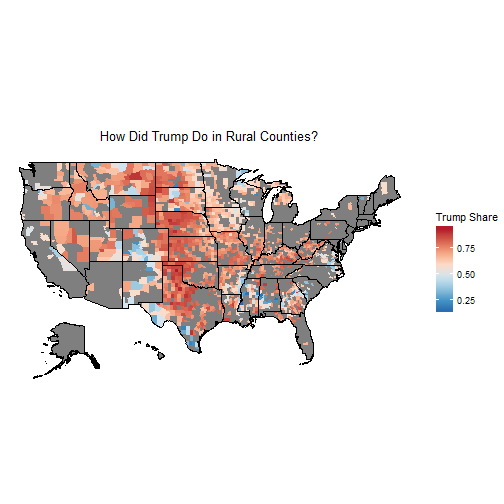
Counties with Above Average Evangelicals
Let’s do the same with evangelicals.
summary(df$evanrate)## Min. 1st Qu. Median Mean 3rd Qu. Max. NA's
## 0.0 107.7 190.5 233.8 334.1 1309.0 18The median here is 190.5 evangelicals per 1000. So any county that’s 19.1% evangelical is in this subset.
high_evan <- filter(df, evanrate >= 190.5)
high_evan$region <- high_evan$fips
high_evan$value <- high_evan$pct
palette_rev <- rev(brewer.pal(8, "RdBu"))
choro = CountyChoropleth$new(high_evan)
choro$title = "                                   Counties with Above Average Evangelicals"
choro$set_num_colors(1)
choro$ggplot_polygon = geom_polygon(aes(fill = value), color = NA)
choro$ggplot_scale = scale_fill_gradientn(name = "Trump Share", colours = palette_rev)
choro$render()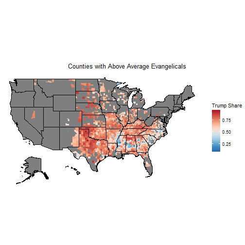
Let’s Combine Rural and High Evangelical
rural_evan <- filter(df, POP2010 <=26080 & evanrate >= 190.5)
rural_evan$region <- rural_evan$fips
rural_evan$value <- rural_evan$pct
palette_rev <- rev(brewer.pal(8, "RdBu"))
choro = CountyChoropleth$new(rural_evan)
choro$title = "                                   Rural Counties with Above Average Evangelicals"
choro$set_num_colors(1)
choro$ggplot_polygon = geom_polygon(aes(fill = value), color = NA)
choro$ggplot_scale = scale_fill_gradientn(name = "Trump Share", colours = palette_rev)
choro$render()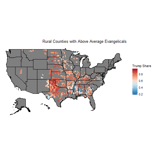
A Searchable Table
table <- select(rural_evan, cntyname, stabbr, pct, POP2010, evanrate)
table$pct <- round(table$pct, 2)
table$evanrate <- round(table$evanrate, 2)
datatable(table, colnames =  c("County", "State", "Trump's Percentage", "2010 Population", "Total Evangelicals per 1000"))
## Error in loadNamespace(name): there is no package called 'webshot'So, how many rural, highly evangelical counties voted for Hillary Clinton?
dim(rural_evan)## [1] 852 11hrc <- filter(rural_evan, pct <=.5)
dim(hrc)## [1] 63 11There were 852 counties in the total dataset and just 63 had a majority of the votes for Clinton. Trump carried 92.6% of those counties.
Suburban, Urban, Rural Data
The CDC provides a classification scheme for urban, suburban, rural. It’s actually six categories:
-
- Large central metro
-
- Large fringe metro
-
- Medium metro
-
- Small metro
-
- Micropolitan
-
- Non-core
Here’s how it breaks down in a map.
df$region <- df$fips
df$value <- df$code
palette_rev <- rev(brewer.pal(8, "RdBu"))
choro = CountyChoropleth$new(df)
choro$title = "                         Urban-Rural Classification Scheme for Counties                                "
choro$set_num_colors(1)
choro$ggplot_polygon = geom_polygon(aes(fill = value), color = NA)
choro$ggplot_scale = scale_fill_gradientn(name = "Rural - Urban", colours = brewer.pal(6, "Spectral"))
choro$render()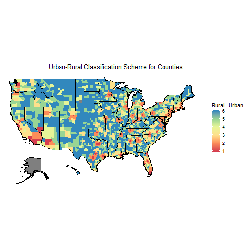
How are evangelicals distributed through these six regions?
a1 <- df %>% group_by(code) %>% summarise(avg_evan = median(evanrate, na.rm = TRUE), trump_vote = median(pct, na.rm = TRUE), total_pop = sum(POP2010, na.rm = TRUE))

a1$code[a1$code==1]<-"Large Central Metro"
a1$code[a1$code==2]<-"Large Fringe Metro"
a1$code[a1$code==3]<-"Medium Metro"
a1$code[a1$code==4]<-"Small Metro"
a1$code[a1$code==5]<-"Micropolitan"
a1$code[a1$code==6]<-"Non-core"
a1$code <- factor(a1$code, levels=unique(a1$code))
ggplot(a1, aes(x=code, y=avg_evan, fill= code)) + geom_col() + xlab("Urban Rural Classification Scheme") + ylab("Number of Evangelicals (per Thousand)") + theme(legend.position="none")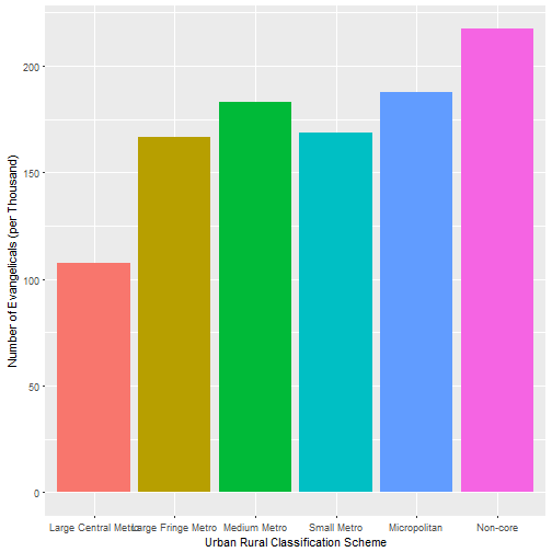
There are definitely more evangelicals in rural areas than in more densely populated areas (by percentage). Large central metros are 10.7% evangelical, and non-core areas are 21.7% evangelical.
ggplot(a1, aes(x=code, y=total_pop/1000000, fill= code)) + geom_col() + xlab("Urban Rural Classification Scheme") + ylab("Total Population (in Millions)") + theme(legend.position="none")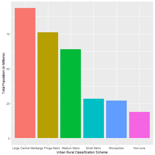
The issue here is that there A LOT more people that live in the metro areas than in the other areas.
a1$evan_percent <- a1$avg_evan/1000
a1$total_evan <- a1$total_pop * a1$evan_percent
a1$percent_total <- a1$total_evan/sum(a1$total_evan)
ggplot(a1, aes(x=code, y=total_evan/1000000, fill= code)) + geom_col() + theme(axis.text.x = element_text(angle = 90)) + theme(legend.position="none") + xlab("Urban Rural Classification Scheme") + ylab("Total Number of Evangelicals (in millions)")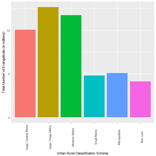
Here’s the upshot of the whole thing. While rural areas are twice as evangelical as the largest metropolitan area, just 8.5% of all evangelicals in the United States live in the “non-core” counties. Even if you add “micropolitan” to “non-core” there are still more evangelicals living in big cities.
Another Table
table2 <- select(a1, code, trump_vote, total_pop, evan_percent, total_evan, percent_total)
table2$percent_total <- round(table2$percent_total, 2)
table2 <- data.frame(table2)
table2 <- table2 %>% rename("Classification" = code, "Trump Vote" = trump_vote, "Total Population" = total_pop, "Percent Evangelical" = evan_percent, "Total Evangelicals" = total_evan, "Percentage of All Evangelicals in Each Classification" = percent_total)
kable(table2)| Classification | Trump Vote | Total Population | Percent Evangelical | Total Evangelicals | Percentage of All Evangelicals in Each Classification |
|---|---|---|---|---|---|
| Large Central Metro | 0.3375237 | 93505527 | 0.1073894 | 10041507 | 0.21 |
| Large Fringe Metro | 0.6030650 | 76007372 | 0.1665800 | 12661308 | 0.26 |
| Medium Metro | 0.5946537 | 63982250 | 0.1833244 | 11729510 | 0.24 |
| Small Metro | 0.6296317 | 28472269 | 0.1689100 | 4809251 | 0.10 |
| Micropolitan | 0.6606895 | 27109461 | 0.1875444 | 5084229 | 0.10 |
| Non-core | 0.7216858 | 18938530 | 0.2174544 | 4118268 | 0.09 |
How Did Trump’s Margins Compare to Romney’s in 2012?
a1<- merge %>% filter(evanrate >250) %>% summarise(mean_trump = mean(trumppct), mean_romney = mean(romneypct))
a2<- merge %>% filter(evanrate >500) %>% summarise(mean_trump = mean(trumppct), mean_romney = mean(romneypct))
a3<- merge %>% filter(evanrate >250 & POP2010 <25000) %>% summarise(mean_trump = mean(trumppct), mean_romney = mean(romneypct))
a4<- merge %>% filter(evanrate >500 & POP2010 <25000) %>% summarise(mean_trump = mean(trumppct), mean_romney = mean(romneypct))
a5 <- rbind(a1, a2, a3, a4)
a5$trump_advantage <- a5$mean_trump - a5$mean_romney
a5$description <- c("25%+ Evangelical", "50%+ Evangelical", "25%+ Evangelical and Population < 25000", "50%+ Evangelical and Population < 25000")
table3 <- a5 %>% rename("Trump Vote Share" = mean_trump, "Romney Vote Share" = mean_romney, "Trump's Margin over Romney" = trump_advantage, "Description" = description)
kable(table3)| Trump Vote Share | Romney Vote Share | Trump’s Margin over Romney | Description |
|---|---|---|---|
| 70.45250 | 66.40706 | 4.045439 | 25%+ Evangelical |
| 75.76940 | 71.30000 | 4.469397 | 50%+ Evangelical |
| 72.86672 | 67.89076 | 4.975959 | 25%+ Evangelical and Population < 25000 |
| 76.76108 | 71.93681 | 4.824279 | 50%+ Evangelical and Population < 25000 |