
Introduction
One day on twitter I saw a tweet that linked to the Movement Advancement Project which provided a tally for how supportive each state was of LGBT rights. I haven’t taken a long time to really dig into the methodology of their index construction, but it seemed like a good jumping off point for doing some data anlaysis.
So, here’s what I wanted to do.
- Work on my scraping skills, especially from websites.
- Understand what’s the best way to combine different datasets that may be slightly different
- Build a Shiny app to display my results.
I thought that would be a nice way to incrementally increase my ability.
Data Cleaning
Try as I might, I really couldn’t find a good way to scrape the LGBT data from their website. Instead I did it the old fashioned way, just plug and chug into an excel sheet. It didn’t take too long, only about 150 entries. In addition I had some other data that I wanted to throw in there. One was a dataset from the ARDA which provides county level religious demography information. In addition, Richard Fording provides state level political ideology scores on his website.
ideo <- read.csv("D:/state_ideo.csv", stringsAsFactors = FALSE)
lgbt <- read.csv("D:/lgbt/lgbt.csv", stringsAsFactors = FALSE)
census <- read.dta("D:/relcensus.dta", convert.factors = FALSE)
Because the religious census data is at the county level, I need to aggregate to the state level instead.
evan <- aggregate(census$evanrate, list(census$stname), mean, na.rm = TRUE)So I want to merge that with my LGBT data. Merge means that I have to create a “key” variable so that R can match the proper rows. Unfortunately that will take a little work. One dataset has the full state name, the other only has the abbreviations. Luckily I found a function online that makes the necessary change.
stateFromLower <-function(x) {
  #read 52 state codes into local variable [includes DC (Washington D.C. and PR (Puerto Rico)]
  st.codes<-data.frame(
    state=as.factor(c("AK", "AL", "AR", "AZ", "CA", "CO", "CT", "DC", "DE", "FL", "GA",
                      "HI", "IA", "ID", "IL", "IN", "KS", "KY", "LA", "MA", "MD", "ME",
                      "MI", "MN", "MO", "MS",  "MT", "NC", "ND", "NE", "NH", "NJ", "NM",
                      "NV", "NY", "OH", "OK", "OR", "PA", "PR", "RI", "SC", "SD", "TN",
                      "TX", "UT", "VA", "VT", "WA", "WI", "WV", "WY")),
    full=as.factor(c("alaska","alabama","arkansas","arizona","california","colorado",
                     "connecticut","district of columbia","delaware","florida","georgia",
                     "hawaii","iowa","idaho","illinois","indiana","kansas","kentucky",
                     "louisiana","massachusetts","maryland","maine","michigan","minnesota",
                     "missouri","mississippi","montana","north carolina","north dakota",
                     "nebraska","new hampshire","new jersey","new mexico","nevada",
                     "new york","ohio","oklahoma","oregon","pennsylvania","puerto rico",
                     "rhode island","south carolina","south dakota","tennessee","texas",
                     "utah","virginia","vermont","washington","wisconsin",
                     "west virginia","wyoming"))
  )
  #create an nx1 data.frame of state codes from source column
  st.x<-data.frame(state=x)
  #match source codes with codes from 'st.codes' local variable and use to return the full state name
  refac.x<-st.codes$full[match(st.x$state,st.codes$state)]
  #return the full state names in the same order in which they appeared in the original source
  return(refac.x)

}
Then I need to convert the other dataset to lower case letters and make the merge.
lgbt$statename<-stateFromLower(lgbt$state)
evan$statename <- tolower(evan$Group.1)
df <- merge(lgbt, evan, by=c("statename"))
Then I realized something. This data isn’t out of order. It’s just the states listed in alphabetical order. Cbind is much simpler because it doesn’t take all the conversion functions. However, the problem is that the some datasets also have Washington, D.C. and/or Puerto Rico. I need to make sure that each is just fifty states.
df <- df[-c(9),]
mainline <- aggregate(census$mprtrate, list(census$stname), mean, na.rm = TRUE)
mainline <- mainline[-c(9),]
mainline$mainline <- mainline$x
mainline <- select(mainline, mainline)
df <- cbind(df, mainline)
What I did then is remove D.C. from both the main dataset (df) and the dataset that contains mainline protestants and then just did cbind. That’s much easier. Then I’m going to do the same with ideology.
ideo <- subset(ideo, year==2014)
ideo$ideology <- ideo$inst6014_nom
ideo <- select(ideo, ideology)
df <- cbind(df, ideo)
df <- select(df, state, orientation, identity, overall, totalpop, popper, x, mainline, ideology)
df$evanrate <- df$x
df$x <- NULL
head(df)
## state orientation identity overall totalpop popper mainline ideology
## 1 AL 2.50 -2.50 0.00 103533 2.8 68.46564 19.058900
## 2 AK 4.25 0.75 5.00 18505 3.4 76.97126 35.443470
## 3 AZ 5.00 -1.75 3.25 192362 3.9 19.38156 3.017494
## 4 AR 4.00 -1.50 2.50 78339 3.5 59.32496 48.899120
## 5 CA 16.00 14.25 30.25 1152048 4.0 23.81355 87.428050
## 6 CO 13.50 9.25 22.75 126599 3.2 63.32743 72.440340
## evanrate
## 1 428.40486
## 2 106.61226
## 3 87.28141
## 4 406.57587
## 5 88.83111
## 6 138.46477So, that’s a good start. Now, I want to add some election results. I found the 2012 presidential election results from the FEC website. Problem is, that data is a mess.
elect <- read.csv("D:/lgbt/elec12.csv", stringsAsFactors = FALSE)
head(elect)
## X obama romney others total
## 1 AL 795,696 1,255,925 22,717 2,074,338
## 2 AK 122,640 164,676 13,179 300,495
## 3 AZ 1,025,232 1,233,654 40,368 2,299,254
## 4 AR 394,409 647,744 27,315 1,069,468
## 5 CA 7,854,285 4,839,958 344,304 13,038,547
## 6 CO 1,323,102 1,185,243 61,177 2,569,522There are commas in there and it’s not numeric. I gotta strip all that out and convert it to numeric before I can cbind it to my main dataframe.
elect$obama <- gsub(',', '', elect$obama)
elect$romney <- gsub(',', '', elect$romney)
elect$others <- gsub(',', '', elect$others)
elect$total <- gsub(',', '', elect$total)
elect$obama <- as.numeric(elect$obama)
elect$romney <- as.numeric(elect$romney)
elect$others <- as.numeric(elect$others)
elect$total <- as.numeric(elect$total)
elect$obama_share <- elect$obama/elect$total
elect$romney_share <- elect$romney/elect$total
elect <- elect[-c(9),]
elect <- select(elect, obama_share, romney_share)
df <- cbind(df, elect)
One last thing. I wanted to grab some state demographic information. I searched for a while before I realized that the best data just comes from Wikipedia tables. So I had to learn some webscraping.
html = read_html("https://en.wikipedia.org/wiki/List_of_U.S._states_by_African-American_population")
aa = html_table(html_nodes(html, "table")[[3]])
aa$percent_AA <- aa$`% African-American`
aa$percent_AA <- as.numeric(sub("%", "", aa$percent_AA))
aa <- select(aa, percent_AA)
df <- cbind(df, aa)

html = read_html("https://en.wikipedia.org/wiki/List_of_U.S._states_by_Hispanic_and_Latino_population")
hisp = html_table(html_nodes(html, "table")[[4]])
hisp$percent_hisp<-hisp$`2012`
hisp <- hisp[-c(1),]
hisp <- hisp[-c(9),]
hisp <- hisp[-c(51),]
hisp <- select(hisp, percent_hisp)
hisp$percent_hisp <- as.numeric(sub("%", "", hisp$percent_hisp))
df <- cbind(df, hisp)
head(df)
## state orientation identity overall totalpop popper mainline ideology
## 1 AL 2.50 -2.50 0.00 103533 2.8 68.46564 19.058900
## 2 AK 4.25 0.75 5.00 18505 3.4 76.97126 35.443470
## 3 AZ 5.00 -1.75 3.25 192362 3.9 19.38156 3.017494
## 4 AR 4.00 -1.50 2.50 78339 3.5 59.32496 48.899120
## 5 CA 16.00 14.25 30.25 1152048 4.0 23.81355 87.428050
## 6 CO 13.50 9.25 22.75 126599 3.2 63.32743 72.440340
## evanrate obama_share romney_share percent_AA percent_hisp
## 1 428.40486 0.3835903 0.6054582 37.30 4.1
## 2 106.61226 0.4081266 0.5480158 32.40 6.1
## 3 87.28141 0.4458977 0.5365453 31.40 30.2
## 4 406.57587 0.3687899 0.6056694 30.10 6.8
## 5 88.83111 0.6023896 0.3712038 28.48 38.2
## 6 138.46477 0.5149215 0.4612698 26.38 21.0To be honest I just had to play around with the html_table command and change the number until it actually grabbed the correct table. Luckily there weren’t too many tables and it only took a few minutes. I cleaned the data and then did cbind it to get it in the correct format.
So, now I we have our data in a manageable format. Let’s do some mapping.
df$region<-stateFromLower(df$state)
df$value <- df$overall
choro = StateChoropleth$new(df)
choro$title = "Support for LGBT Rights"
choro$set_num_colors(1)
choro$ggplot_polygon = geom_polygon(aes(fill = value), color = NA)
choro$ggplot_scale = scale_fill_gradientn(name = "Overall Tally", colours = viridis(32))
choro$render()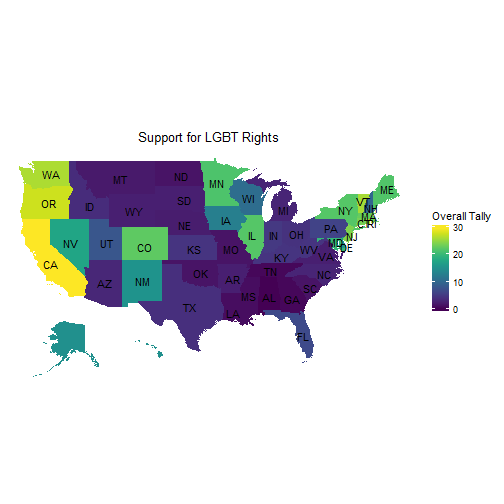
The south is not the best place to live if you are LGBT. The Pacific coast states are the most supportive, followed by New England. There is a surprising amount of support in the upper Midwest including Illinois, Wisconsin, Iowa, and Minnesota.
Let’s do a little regressing to look for relationships.
df$region <- NULL
df$value <- NULL
reg1 <- lm(overall ~ totalpop + popper + ideology + evanrate + mainline + ideology + obama_share + romney_share + percent_AA + percent_hisp, data =df)
summary(reg1)
##
## Call:
## lm(formula = overall ~ totalpop + popper + ideology + evanrate +
## mainline + ideology + obama_share + romney_share + percent_AA +
## percent_hisp, data = df)
##
## Residuals:
## Min 1Q Median 3Q Max
## -8.8023 -2.4612 0.2235 2.4692 6.7007
##
## Coefficients:
## Estimate Std. Error t value Pr(>|t|)
## (Intercept) 1.377e+01 9.576e+01 0.144 0.8864
## totalpop 1.370e-06 4.082e-06 0.336 0.7389
## popper 1.204e+00 1.212e+00 0.994 0.3263
## ideology 1.569e-01 3.119e-02 5.031 1.07e-05 ***
## evanrate -1.636e-02 6.836e-03 -2.393 0.0215 *
## mainline 6.294e-04 1.020e-02 0.062 0.9511
## obama_share -3.001e+00 9.479e+01 -0.032 0.9749
## romney_share -2.349e+01 9.946e+01 -0.236 0.8145
## percent_AA -5.460e-02 6.923e-02 -0.789 0.4350
## percent_hisp 2.126e-01 8.548e-02 2.487 0.0172 *
## ---
## Signif. codes: 0 '***' 0.001 '**' 0.01 '*' 0.05 '.' 0.1 ' ' 1
##
## Residual standard error: 4.414 on 40 degrees of freedom
## Multiple R-squared: 0.832, Adjusted R-squared: 0.7943
## F-statistic: 22.02 on 9 and 40 DF, p-value: 7.719e-13Just two things predict higher LGBT support. State ideology, which makes sense. The other is percent hispanic. That may not be because of hispanics specifically but because hispanics tend to migrate to states that are already liberal such as California. One negative predictor is the number of evangelicals.
I wanted to make this into an interactive Shiny app. I had to make some conversions in my data and build a ui.R file, along with a server.R file. Those can be found in my Github account.
The Shiny app can be accessed at https://ryanburge.shinyapps.io/Predicting_LGBT_Rights/. It includes the ability to generate a regression line as well a correlation between the two values chosen. Possible X variables include the overall tally, the sexual orientation tally, and the gender identity tally. The Y axis contains all the variables contained in the regression that I just displayed.