
Load a few packages
library(ggplot2)
library(readr)
library(dplyr)
library(ggvis)
Read in my data
names <- read.csv("D:/NationalNames.csv", stringsAsFactors = FALSE)I am looking for a name that is quintessential hipster name. Here are the criteria:
- Very popular 100 years ago
- Very unpopular 30 years ago
- Becoming much more popular in the last five years
I started by looking for a name that seems to follow that pattern - Hazel.
hazel <- subset(names, Name == "Hazel" & Gender =="F")
hazel  %>%
select (Name, Year, Count) %>%
ggvis(~Year, ~Count, stroke = ~factor(Name)) %>%
layer_lines()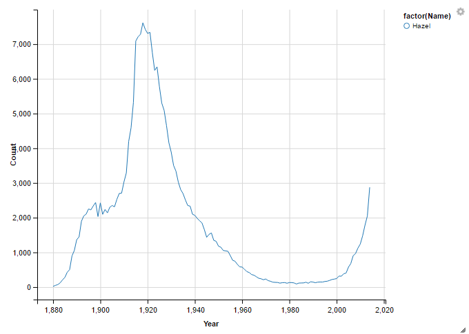
That’s a great start. Hazel reached it’s peak popularity in the late 1910’s and then declined sharply, now it’s back. Let’s try another guess to look for good count thresholds.
violet <- subset(names, Name == "Violet" & Gender =="F")
violet  %>%
select (Name, Year, Count) %>%
ggvis(~Year, ~Count, stroke = ~factor(Name)) %>%
layer_lines()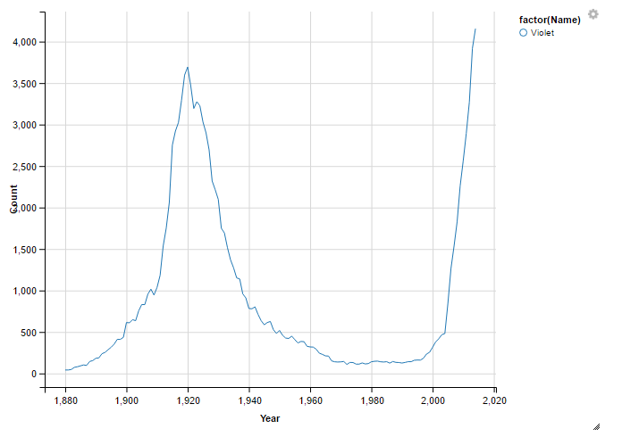
Both names seem to have the same trend.
- At least 3000 at some point between 1915 and 1930
- Less than 1000 around 1980
- More than 2000 at any point after 2010.
That’s the criteria I want to use to look for those names.
df1 <- subset(names , Gender =="F" & Year >= 1915 & Year <= 1935 & Count > 3000)
df2 <- subset(names, Gender == "F" & Year == 1980 & Count <= 1000)
df3 <- subset(names , Gender == "F" & Year >= 2010 & Year <= 2014 & Count > 2000)
Created three data frames to match my criteria.
Now, let’s see how many names will be charted
names   %>%
filter(Gender == 'F', Name %in% df1$Name, Name %in% df2$Name, Name %in% df3$Name)  %>%
select (Name, Year, Count) %>%
ggvis(~Year, ~Count, stroke = ~factor(Name)) %>%
layer_lines()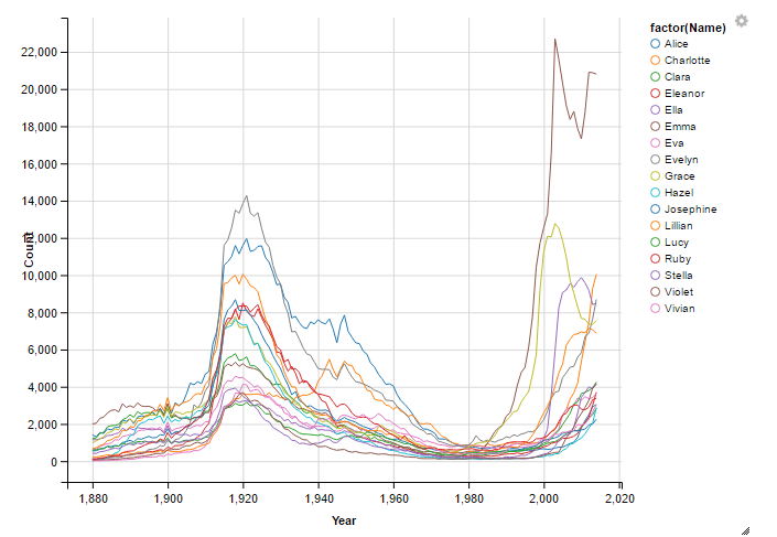
That’s a solid set of names and many seem to fit into the mold that I was envisioning.
Let’s try the same with boy’s names.
df4 <- subset(names , Gender =="M" & Year >= 1915 & Year <= 1935 & Count > 3000)
df5 <- subset(names, Gender == "M" & Year == 1980 & Count <= 1000)
df6 <- subset(names , Gender == "M" & Year >= 2010 & Year <= 2014 & Count > 2000)
names   %>%
filter(Gender == 'M', Name %in% df4$Name, Name %in% df5$Name, Name %in% df6$Name)  %>%
select (Name, Year, Count) %>%
ggvis(~Year, ~Count, stroke = ~factor(Name)) %>%
layer_lines()
Well, that’s a much different outcome than I was looking for. Just one name.
I tried to add more names by changing several of each Count threshold.
df4 <- subset(names , Gender =="M" & Year >= 1915 & Year <= 1935 & Count > 1500)
df5 <- subset(names, Gender == "M" & Year == 1980 & Count <= 1000)
df6 <- subset(names , Gender == "M" & Year >= 2010 & Year <= 2014 & Count > 1000)
names   %>%
filter(Gender == 'M', Name %in% df4$Name, Name %in% df5$Name, Name %in% df6$Name)  %>%
select (Name, Year, Count) %>%
ggvis(~Year, ~Count, stroke = ~factor(Name)) %>%
layer_lines()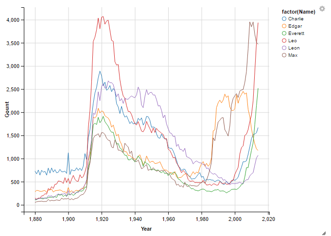
Thanks to a nice comment from FlorianGD, I realized that by halving the lower threshold in df5 I actually made it harder rather than easier for a name to show up. This moved my total number of boys names from 3 to 6. That’s reflected in the new figure above.