
Packages and Data Import
Here I am going to load the packages that I need and then import the Paul Simon dataset that I am using.
A link to the codebook can be found here
#install.packages("ggplot2")
#install.packages("car")
#install.packages("dotwhisker")
library(ggplot2)
library(car)
library(dotwhisker)
simon <- read.csv(url("http://goo.gl/exQA14"))
Recoding
We are going to run an OLS regression to predict support for Governor Bruce Rauner, that is our dependent variable. Then we are going to have a number of independent variables including party identification, gender, union membership, region of the state, age, and income.
Before we get to the regression, we have to do some preliminary steps. One of the most important things that you must do before you run a regression is to clean your data.
simon$rauner <- recode(simon$app_gov_rau, "9=3")
simon$rauner <- recode(simon$rauner, "1=5; 2=4; 3=3; 4=2; 5=1; else=0")
simon$partyid <- recode(simon$party_leans, "8=0; 9=0")
simon$male <- recode(simon$gender, "2=0")
simon$labor <- recode(simon$union, "1=1; else=0")
simon$downstate <- recode(simon$area, "3=1; else=0")
simon$age <- 2016 - simon$birth_yr
simon$age <- recode(simon$age, "116=0")
simon$income <- recode(simon$hhinc, "8=0; 9=0")
I am basically dumping a lot of the “don’t know” responses to zero so that they don’t mess up our analysis. It’s important to be consistent with how you deal with DK responses. Make sure to describe how you do that so that you can remember later on.
OLS Regression
So, let’s get to the regression part. We are going to use the lm() function from R to construct a linear model. It is going to create an output called reg1. When you run the first command, notice that nothing will happen. If you want to actually see the output in table format, use the summary() command.
reg1 <- lm(rauner ~ partyid + age + labor + income + downstate + male, data = simon)
summary(reg1)
##
## Call:
## lm(formula = rauner ~ partyid + age + labor + income + downstate +
## male, data = simon)
##
## Residuals:
## Min 1Q Median 3Q Max
## -3.2658 -1.1074 0.0064 1.0575 3.4993
##
## Coefficients:
## Estimate Std. Error t value Pr(>|t|)
## (Intercept) 1.856e+00 1.441e-01 12.879 < 2e-16 ***
## partyid 2.955e-01 2.027e-02 14.578 < 2e-16 ***
## age -4.822e-05 1.999e-03 -0.024 0.980760
## labor -4.173e-01 1.071e-01 -3.897 0.000104 ***
## income -2.300e-02 1.868e-02 -1.231 0.218587
## downstate -1.879e-01 9.673e-02 -1.943 0.052331 .
## male 3.445e-01 8.750e-02 3.937 8.82e-05 ***
## ---
## Signif. codes: 0 '***' 0.001 '**' 0.01 '*' 0.05 '.' 0.1 ' ' 1
##
## Residual standard error: 1.356 on 993 degrees of freedom
## Multiple R-squared: 0.2232, Adjusted R-squared: 0.2185
## F-statistic: 47.55 on 6 and 993 DF, p-value: < 2.2e-16dwplot(reg1) + geom_vline(xintercept = 0, colour = "grey50", linetype = 2)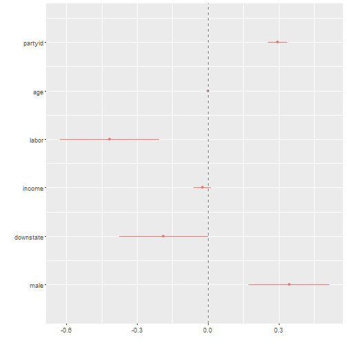
So, what you see is a regression output. Each of indepedent variables are listed in the far left column. Then there is the estimate in the second column. Finally, look at the far right? Those are the statistical significance stars. If a row doesn’t have stars, then that relationship is not statistically significant. For example, our DV is Rauner’s approval rating. Look at the age variable. You see how there are no stars there? That means that there is not a statistical relationship between the two things.
One interpretation thing. I had to reverse code the Rauner variable so that higher values is more approval and lower values are less approval. The codebook has it backwards.
Look at the dotwhisker plot I made. Here’s how you interpret that. If that dot or the horizontal red line’s overall with the vertical dashed line, then those variables are not statistically significant. If the dot is to the right and doesn’t overlap zero then it’s positively related, if it’s to the left and doesn’t overlap zero then it is negative. So, we can see that being a member of a labor union has a strong negative impact on Rauner’s approval rating. In fact, we can say that being a member of a union decreases his approval by about ten percent.
Add Black
Let’s add a racial component. I will create a dichtomous variable for black and then add it to the regression I just ran.
simon$black <- recode(simon$rac_eth, "2=1; else=0")
reg2 <- lm(rauner ~ partyid + age + labor + income + downstate + male + black, data = simon)
summary(reg2)
##
## Call:
## lm(formula = rauner ~ partyid + age + labor + income + downstate +
## male + black, data = simon)
##
## Residuals:
## Min 1Q Median 3Q Max
## -3.2873 -1.1171 0.0337 1.0614 3.4548
##
## Coefficients:
## Estimate Std. Error t value Pr(>|t|)
## (Intercept) 2.0205179 0.1506120 13.415 < 2e-16 ***
## partyid 0.2834446 0.0204428 13.865 < 2e-16 ***
## age -0.0003402 0.0019892 -0.171 0.864239
## labor -0.4069261 0.1065082 -3.821 0.000141 ***
## income -0.0275496 0.0186194 -1.480 0.139292
## downstate -0.2476426 0.0976417 -2.536 0.011357 *
## male 0.3105896 0.0875206 3.549 0.000405 ***
## black -0.4758912 0.1343286 -3.543 0.000414 ***
## ---
## Signif. codes: 0 '***' 0.001 '**' 0.01 '*' 0.05 '.' 0.1 ' ' 1
##
## Residual standard error: 1.348 on 992 degrees of freedom
## Multiple R-squared: 0.2329, Adjusted R-squared: 0.2275
## F-statistic: 43.02 on 7 and 992 DF, p-value: < 2.2e-16dwplot(reg2) + geom_vline(xintercept = 0, colour = "grey50", linetype = 2)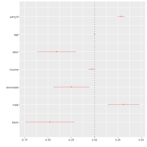
What changes here? What stays the same? Obviously being black is negatively correlated to supporting Rauner. However, we cannot say whether being in a union is more or less powerful than being black when it comes to supporting the Governor because their confidence intervals overlap each other. Same can be said for partyid and male gender.
Logit Regression
We use the lm() command because our variable (Governor Rauner’s support) had five possible values 1,2,3,4,5. However, what happens if your dependent variable is dichotomous and therefore has only 2 values? You would have to run a logit. The DV we are looking at here is support for recreational marijuana. I have recoded it so that 1 is supporting the proposal and every other response is a zero in the dataset. Then I will run a logit regression with the glm() command and the same IVs as the previous analysis.
simon$mjrec <- recode(simon$mari_rec, "1=1; else=0")
reg1 <- glm(mjrec ~ partyid + age + labor + income + downstate + male + black, data = simon)
summary(reg1)
##
## Call:
## glm(formula = mjrec ~ partyid + age + labor + income + downstate +
## male + black, data = simon)
##
## Deviance Residuals:
## Min 1Q Median 3Q Max
## -0.9087 -0.4284 -0.2003 0.4773 0.9098
##
## Coefficients:
## Estimate Std. Error t value Pr(>|t|)
## (Intercept) 0.6234167 0.0531105 11.738 < 2e-16 ***
## partyid -0.0333467 0.0072088 -4.626 4.22e-06 ***
## age -0.0040032 0.0007015 -5.707 1.52e-08 ***
## labor 0.0387214 0.0375581 1.031 0.302804
## income 0.0288631 0.0065658 4.396 1.22e-05 ***
## downstate -0.0497403 0.0344315 -1.445 0.148882
## male 0.1022945 0.0308625 3.315 0.000951 ***
## black 0.0359730 0.0473684 0.759 0.447776
## ---
## Signif. codes: 0 '***' 0.001 '**' 0.01 '*' 0.05 '.' 0.1 ' ' 1
##
## (Dispersion parameter for gaussian family taken to be 0.2259264)
##
## Null deviance: 247.50 on 999 degrees of freedom
## Residual deviance: 224.12 on 992 degrees of freedom
## AIC: 1360.3
##
## Number of Fisher Scoring iterations: 2dwplot(reg1) + geom_vline(xintercept = 0, colour = "grey50", linetype = 2)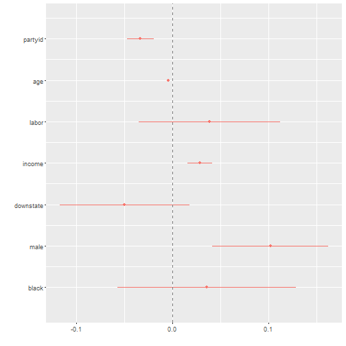
We can see here that there are only a few statistically significant variables. Age, partyid, income, and male. The partyid variable ranges from zero to 7. That’s eight total values. Each step up that scale (toward Republican ID) makes someone 3.3% less likely to support recreational marijuana. Being male makes you 10% more likely to support the proposal, however.